Generative Design Computing . Sharpe - Project 4

This project was an assignment to create a parametric truss system and have it spanning along a large surface. I was also interested in seeing how it would perform on a complex/irregular/non-uniform single surface.

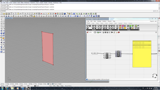
The first step is to begin building a basic truss on a rectangular surface. First we set a Surface function and attach that to a Surface Divide function. In order to get 4 corner points, we set the SDivide function's U and V value at 1. We then attach a Simplify function along with a notepad to confirm that we have correctly setup the points, and into 2 different categories.

The next step is set up 2 different branches which will separate the points into 2 groups. The top Branch is set to receive the points from category 0, while the bottom Branch will receive points from category 1 - this is achieved by setting P to 0 for the top and 1 for the bottom Branch. The branches are further broken down into single points by using the Item functions and setting the integer (i) values to 0 and 1 for each of the two branches.

Once the individual items were set, we assign a single Point to each Item. The next step was to create a solid polyline and a plane using 3 points. By using the PLine function, we attach 3 points to create the closed polyline and the Plane 3pt function determines the plane that the polyline lies on. All of the these functions are done twice to create 2 different triangles that bisect the rectangular surface. Once the polylines are created, we can offset them by using the Offset function, attaching the polylines as the input curves and using the Plane 3pt as the plane in which to offset. By attaching a slider we are able to control the distance of the offset, and if the offset is in the wrong direction we can set a -d expression to reverse the offset side.

The last step with the single surface truss is to set a Fillet function with a slider to adjust the fillet radius. We then attach this polyline with the original perimeter triangle geometry into a Join function. The final step is to assign a Planar function to create surface between the perimeter trinagle and the offset polyline.

The second half of this tutorial is to show the steps of how to assign the single surface truss onto a large and comnplex surface. After creating the complex surface, we assign it to a Surface parameter and plug that into a Divide and into a SubSrf (Isotrim) function. The Divide function has numeric sliders to control the amounts of divisions in the U and V directions. This is then plugged into a SDivide function to add points at the corners - the U and V values must be set to 1 to achieve this. Finally a Simplify function is added to eliminate overlapped/redundant points.




Now we use this new surface and all of its divisions and replace the original single surface and the components - everything up to the first, original notepad.




The next step is to use a Param Viewer function in order to take the detailed information and translating this into individual paths - info from the first notepad is the input data for the Param Viewer. We use a notepad to see the list of the newly translated individual paths, and then plug these into two different Item functions. The Item functions are then plugged back into the original Branch path slots (P).



The final step is to insert a Series and Multiply function and to insert the surface's division sliders into the Multiply function. This will all for an accurate number of individual trusses to be applied to the U and V subsurfaces that have been created by the division. The Multiply function is plugged into the Series, and the Series is then plugged into both of the Item functions.

This is the final output geometry with 10x10 divisions and an offset of 1.1.

This is the final output geometry with 22x22 divisions and an offset of .02.

Generative Design Computing . Sharpe - Project 3

This project was developed using a Morph Tile definition written in Grasshopper and a requirement of the project was to produce a 3D print of the object that we created in Rhino. I began by developing a series of lines that would unfold, twist, shrink and expand the surface of the object.




At the beginning of the Grasshopper definition, I assigned all curves to the Curve function and lofted them. I setup a Divide function along with a Isotrim function, which divides surfaces into individual surfaces.

This is where a Surface Box definition was added to create three-dimensional twisted boxes from the individual surfaces. The Area function was added to analyze the area of each surface, which is attached to a 2-Function definition, set as x>y. Notepads were added to the Area and F2 functions to see the results.

Two solid objects were created in Rhino to be used as the surface patterns. One object has an opening in the middle and the other object is closed. A Dispatch function was added to separate the True and False values created from the F2 function.




The final section of the Grasshopper definition is where the Dispatch information plugs into two different Box Morphs. The open solid geometry is attached to one Bounding Box function, and then into one Morph Box while the closed solid geometry is attached to the other Bounding Box and Morph Box. Essentially, the two different tile geometries are distributed throughout the surface, with the open geometry assigned to the larger areas, and the closed geometry assigned to the smaller areas. This is the final object that was used to create a 3D print.

The following images are of the 3D print model.



Generative Design Computing . Sharpe - Project 2

This project required us to create a Grasshopper model that allows for parametric control of objects. I created a simple model that includes a geometry arranged on a grid, along with an attractor point that resizes the geometry.

I began by setting up a Square Grid and attaching sliders. The first slider controls the distance between grid points, and the second and third slider controls the number of rows and columns.

The next step was inserting a Distance variable, and this will determine the distance between the grid points and a floating point. This floating point was created in Rhino and linked in Grasshopper. Then I put in a Division variable which will cause objects near the attractor point to decrease in size.

The final step in the Grasshopper model was to define the geometry at each grid points. I inserted a Polygon definition that has the grid points and the attractor point variables. The polygon includes a slider plugged in to change the shape (number of sides) of the polygons.

Examples of final images created after baking the Grasshopper model and filling in the geometry in Adobe Illustrator.

13x13 grid, 3-sided geometry and attractor point in the lower left corner.

13x14 grid, 4-sided geometry, attractor point in the upper right corner.

16x11 grid, 6-sided geometry, grid spacing was enlarged, attractor point in the center.

16x16 grid, 50-sided geometry (circle), grid spacing was condensed, attractor point in bottom right corner.

Generative Design Computing . Sharpe - Project 1

I wanted to develop an object with a lot of curvature and my project began with this linework.

After using the loft command this is the surface that was produced.

Using the Paneling Tools menu, I created a grid by using "Surface Domain" and then used "Offset Points" to offset the grid.

I then created panels with different configurations in order to produce geometry with variation. Using the "Panel Custom 3D Variable" command, I selected the grids and panels, and then setup Attractor Points.

This is the panel geometry that was produced.

In order to get a useful surface for laser cutting I had to explode the solids and choose 1 side of the panels to preserve.

Once I unrolled the surface using "Unroll Faces", I had to manipulate the output to be sure that it would properly be cut on the laser cutter. First, I had to separate the overlapping pieces and then change the colors - Red for a full cut and Black for an etching (surface cut which will allow the chipboard to flex).



This is an image of the chipboard after laser cutting.

These are images of the final model completely assembled.

Test Post 001

this is the first post of the term